What Gemma 4 Actually Does Differently

Gemma 4's 31B model is outscoring GPT-4 class systems on Arena Elo — models with 10× more parameters. Kimi k2.5 runs 1100B. Qwen 3.5 runs 397B. GLM-5 runs 754B. Gemma 4 31B sits at 1452, ahead of most of them.

So what's actually going on here?

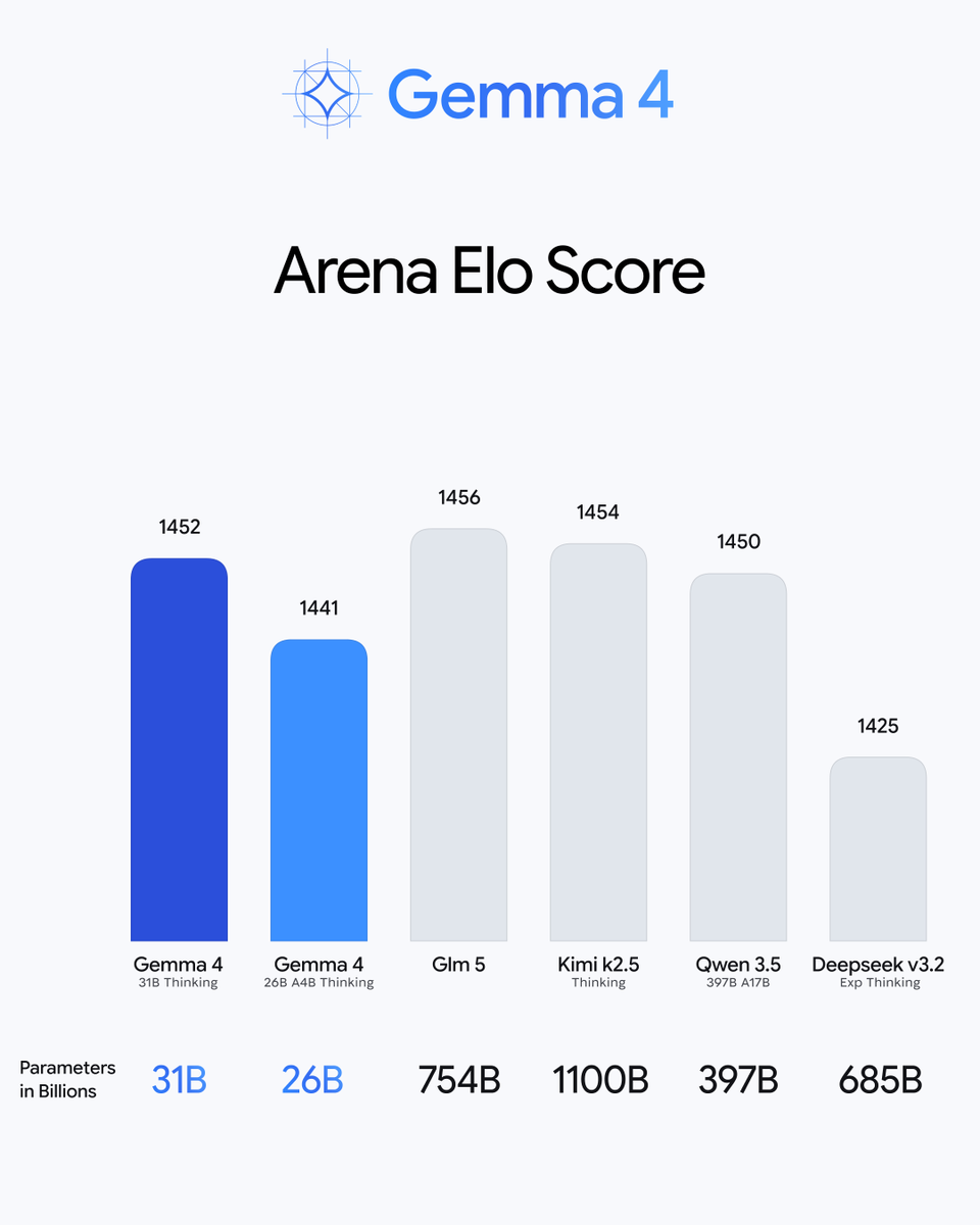Gemma 4 31B scoring 1452 Elo against models ranging from 26B to 1100B parameters.

Four models, one philosophy

Gemma 4 isn't one model — it's four, built for very different situations. E2B and E4B are the tiny ones that can run on a phone and handle text, images, and audio. 31B is a large dense model — straightforward architecture, needs a real GPU. 26B A4B is the interesting one: 26 billion parameters total, but only 4 billion are used per token, thanks to Mixture of Experts. More on that later.

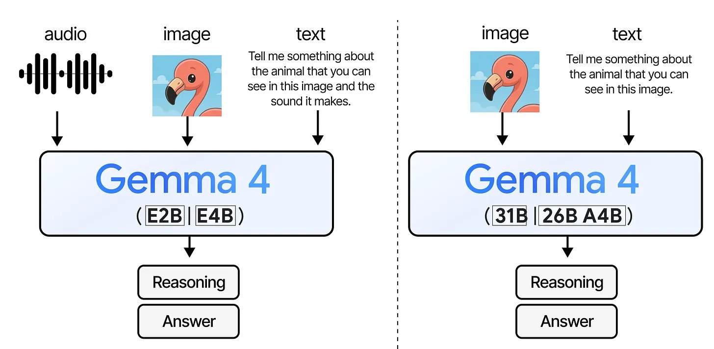All four models take images and text. E2B and E4B also take audio — the bigger ones don't. — Maarten Grootendorst

All four models are multimodal — they understand both text and images natively. The two small ones go further and also take audio as input, which opens up things like on-device speech recognition without needing a separate model for it.

What connects the family isn't just shared code — it's a shared obsession. Every design decision in Gemma 4 is about finding a specific place where compute or memory is being wasted, and surgically fixing it. That's what most of this post is about.

Most attention is local (and that's the point)

Attention is where a Transformer spends most of its time. In full (global) attention, every token compares itself against every other token in the sequence. It's thorough, but the cost grows quadratically — double the context length and you quadruple the work.

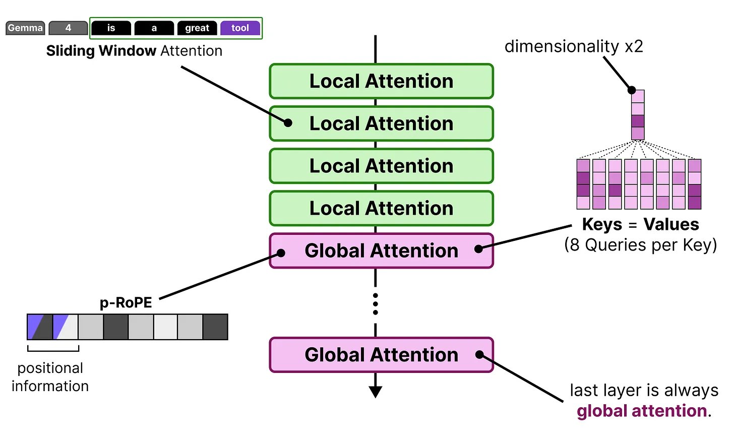
Gemma 4 sidesteps this by making most layers use sliding window attention. Instead of looking at the entire sequence, each token only looks at the nearest 512 tokens (or 1024 for the bigger models). The cost becomes linear with the window size, not the full sequence length. For a model processing tens of thousands of tokens, this is a massive difference.

The obvious downside: if you can only see the last 512 tokens, you lose track of things that happened earlier. So every 5th or 6th layer, Gemma 4 runs a global attention layer where every token can see everything. These layers are expensive, but they only fire occasionally — maybe 10 out of 60 layers in the 31B model.

Gemma 3 already did this. What Gemma 4 changed is small but matters: the last layer is always global. In Gemma 3, the interleaving pattern could land a local layer at the end, which meant the model's final representation — the one that actually generates the output — might not have full visibility over the context. That's now fixed.

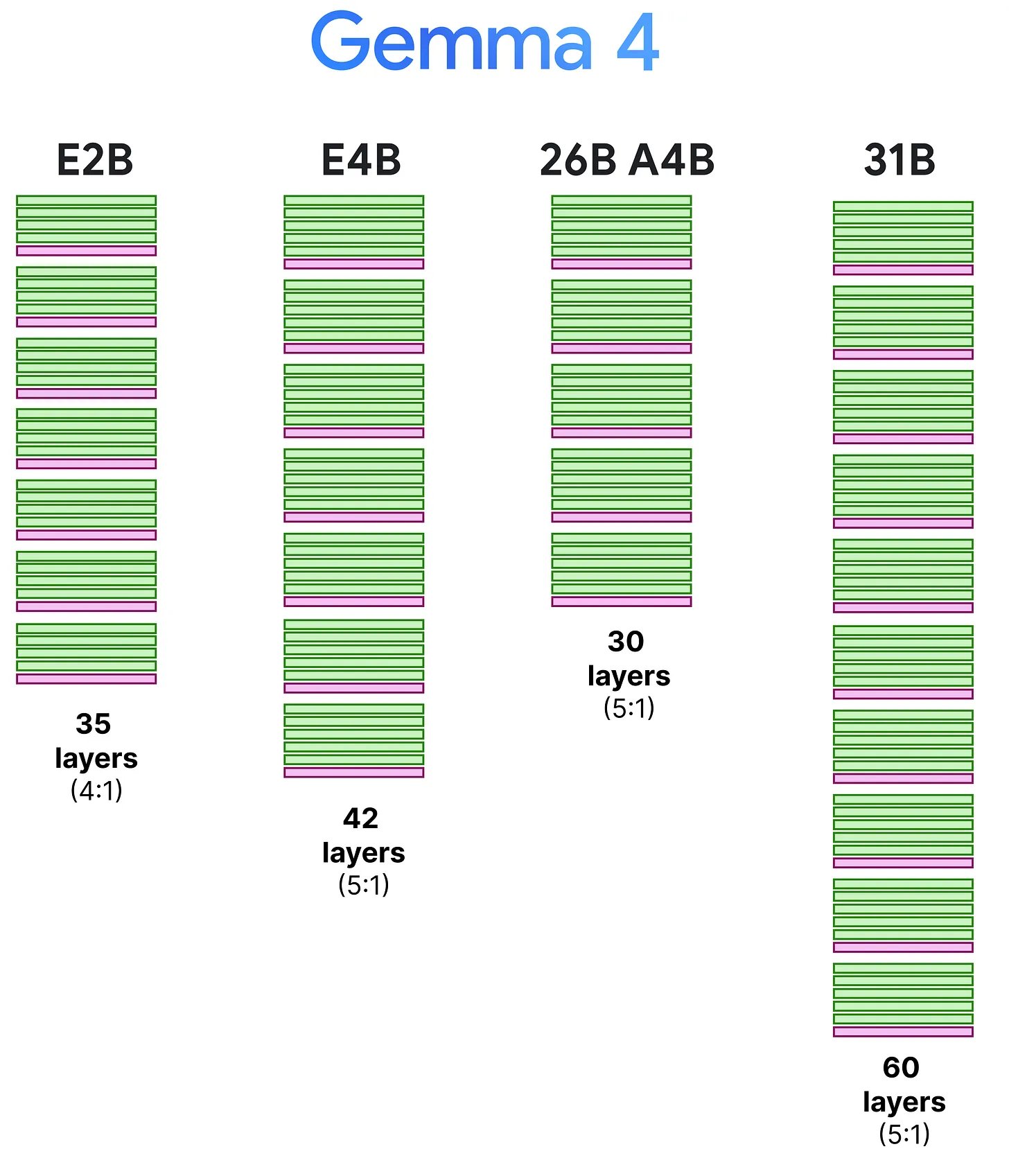Green = local attention, pink = global attention. Every model ends on a global layer. — Maarten Grootendorst

The global layers are still expensive — so Gemma 4 makes them cheaper

Interleaving is great, but you still have those global layers attending to the full context. In a model with a 128k token context window, that's a lot of Key-Value pairs to cache and compute over. Gemma 4 applies three techniques here, and they all target the same bottleneck: the KV-cache of the global layers.

More sharing in Grouped Query Attention

Quick refresher: in attention, each token produces a Query ("what am I looking for?"), a Key ("what am I about?"), and a Value ("here's my content"). Grouped Query Attention lets multiple Query heads share the same Key-Value pair, which means fewer KV pairs to store.

The local layers in Gemma 4 use a 2:1 ratio — two Query heads per KV pair. The global layers crank it up to 8:1. That's four times less KV storage per layer, which matters a lot when the global layer is caching the entire context.

The tradeoff is that with fewer KV heads, each one needs to carry more information. So the Key dimensions are doubled from 256 to 512. You're storing fewer Keys, but each Key is richer.

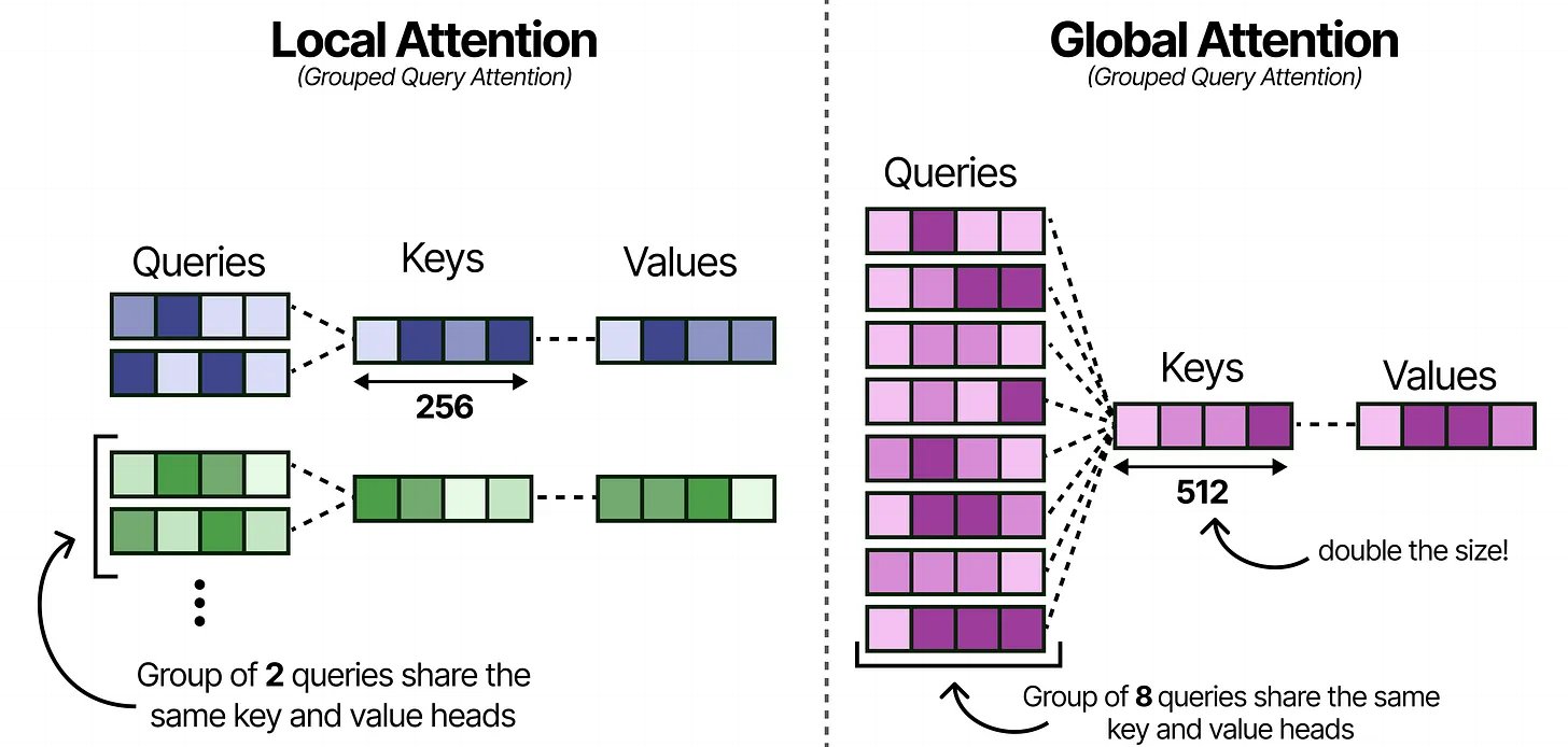Local layers share at 2:1, global layers at 8:1 — fewer KV pairs, but each Key is doubled in size to compensate. — Maarten Grootendorst

Keys = Values

This one is elegant. In the global layers, Gemma 4 sets the Keys and Values to be the same tensor. Normally you'd store both a K-cache and a V-cache for every token in the context. With K=V, you store one.

Why does this work at all? In practice, the Keys already contain a compressed representation of each token — what it's "about." The Values are supposed to hold the actual content to pass forward. Making them identical sounds like it should hurt, but empirically the quality loss is minimal. The model apparently learns to pack enough information into a single representation to serve both roles. And you get a roughly 2× reduction in cache memory for the global layers, which is where memory pressure is worst.

p-RoPE: stop adding noise to the dimensions that carry meaning

This one requires a bit of setup. RoPE (Rotary Positional Encoding) is how the model knows word order. It works by rotating pairs of values in the Query and Key embeddings — each pair gets rotated by an amount that depends on the token's position in the sequence. The first pair gets a large rotation (high frequency), the last pair gets a tiny one (low frequency).

Here's what happens in practice: the high-frequency pairs encode position well, but the low-frequency ones barely rotate at all — even across hundreds of tokens, the rotation is negligible. They end up carrying almost no positional information. Instead, the model learns to use those dimensions for semantic content — what a word means rather than where it is.

The problem is that standard RoPE still applies a small rotation to those dimensions. Over short contexts, this noise is harmless. Over long contexts — say, 128k tokens — those tiny rotations accumulate and start interfering with the semantic information the model stored there. Tokens that are far apart can end up with rotations that look confusingly similar, making it harder for the model to distinguish their meanings.

p-RoPE just removes the rotation from those dimensions entirely. In Gemma 4, only the first 25% of dimension pairs get positional encoding. The other 75% get zero rotation — they're purely semantic. This is applied to the global layers specifically, where the long context makes the noise problem worst.

It's a small change, but it's the kind of thing that compounds: cleaner representations → better long-range connections → better output quality on long inputs.

GQA + K=V + p-RoPE stacked — three separate fixes targeting the same global attention bottleneck. — Maarten Grootendorst

None of these three techniques are individually novel — you can find papers on each. What's notable is stacking them. They target different aspects of the same bottleneck (GQA reduces the number of KV pairs, K=V halves the per-pair storage, p-RoPE improves what the remaining dimensions encode) and they compose without fighting each other.

How images get processed

All four models can take images as input. The approach is Vision Transformer (ViT) — the image gets chopped into a grid of 16×16 pixel patches, each patch gets projected into an embedding, and those embeddings are processed by a Transformer encoder. The output is a set of "visual tokens" that represent the image.

What's different in Gemma 4 is the flexibility. Two things stand out:

Variable aspect ratios. Most vision models resize every image into a fixed square before processing. That's fine for profile photos, but a panoramic landscape or a tall screenshot gets distorted. Gemma 4 instead adapts the grid to match the image's actual shape and uses 2D RoPE (separate positional encoding for width and height) so the model understands spatial relationships regardless of aspect ratio. Padding is added where the image doesn't perfectly tile into 16×16 patches.

Controllable resolution. The model exposes a "soft token budget" — you choose between 70, 140, 280, 560, or 1120 visual tokens. This controls how much the image is downscaled before patching. For a task like captioning, 70 tokens might be enough. For reading small text in a document image, you'd want 1120. This is a practical knob that lets you trade quality for speed depending on your actual task.

After the ViT produces patch embeddings, neighbouring patches are merged in 3×3 blocks (averaged) to bring the count down, then a linear projection + RMSNorm transforms them to match the language model's embedding space. At that point, image tokens and text tokens sit side by side in the same sequence and get processed together.

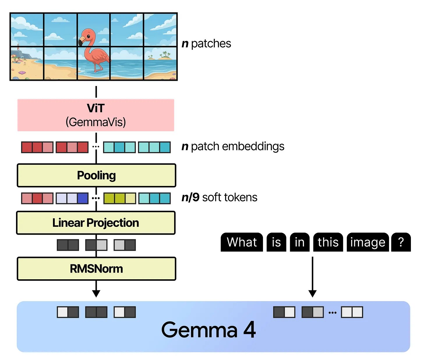Image → patches → ViT → pooling → projection → lands in the same sequence as text tokens. — Maarten Grootendorst

Mixture of Experts: the 26B A4B model

In a normal (dense) Transformer, every layer has one feedforward network and every token goes through all of it. In the 26B A4B model, that feedforward network is replaced by 128 smaller expert networks and a router.

When a token arrives at an MoE layer, the router looks at it and picks 8 of the 128 experts to activate. Only those 8 do computation for that token — the other 120 are completely idle. The router also assigns each selected expert a weight, so some experts have more influence on the output than others.

There's also a shared expert that runs on every token regardless. It's 3× larger than a regular expert and acts as the general-purpose backbone — the knowledge that's useful no matter what the token is about. The routed experts, by contrast, tend to specialise. During training, different experts naturally develop expertise in different kinds of tokens or patterns.

The practical result: you need enough memory to load all 26 billion parameters (all 128 experts have to be in memory because you don't know which ones the router will pick). But the compute per token only involves the 8 selected experts plus the shared one — roughly 4 billion active parameters. The model runs at about the speed of a 4B dense model while having access to 26B worth of learned knowledge.

This is why the name is "26B A4B" — 26 billion total, 4 billion active.

Per-Layer Embeddings: the phone models

E2B and E4B have a different efficiency problem. On a phone, you don't have a lot of RAM, and you need most of what you have for the model's computation — the matrix multiplications that happen in attention and the feedforward layers. Anything you can get out of RAM is valuable.

Normally, a model has a big embedding table at the bottom — a lookup that maps each token in the vocabulary (262,144 tokens in Gemma 4's case) to a dense vector. This table sits in RAM. What the E-models do is create an additional set of smaller embeddings for every token at every layer, and store that whole table in flash storage instead of RAM.

Flash storage is what your phone's SSD is — it's much cheaper and more plentiful than RAM, but slower to access randomly. The trick is that PLE only needs to be read once: at the start of inference, the model fetches all the per-layer embeddings for every token in your prompt in a single batch read. After that, no more flash accesses are needed.

At each layer, the model takes the corresponding PLE, runs it through a gating function (so it can learn which parts of the embedding to emphasise), projects it up from 256 dimensions to the model's full hidden size (1536 for E2B), and adds it to the main hidden state. The effect is that the model gets a token-specific signal injected at every layer, reminding it of what each token originally meant — even after many layers of attention have mixed everything together.

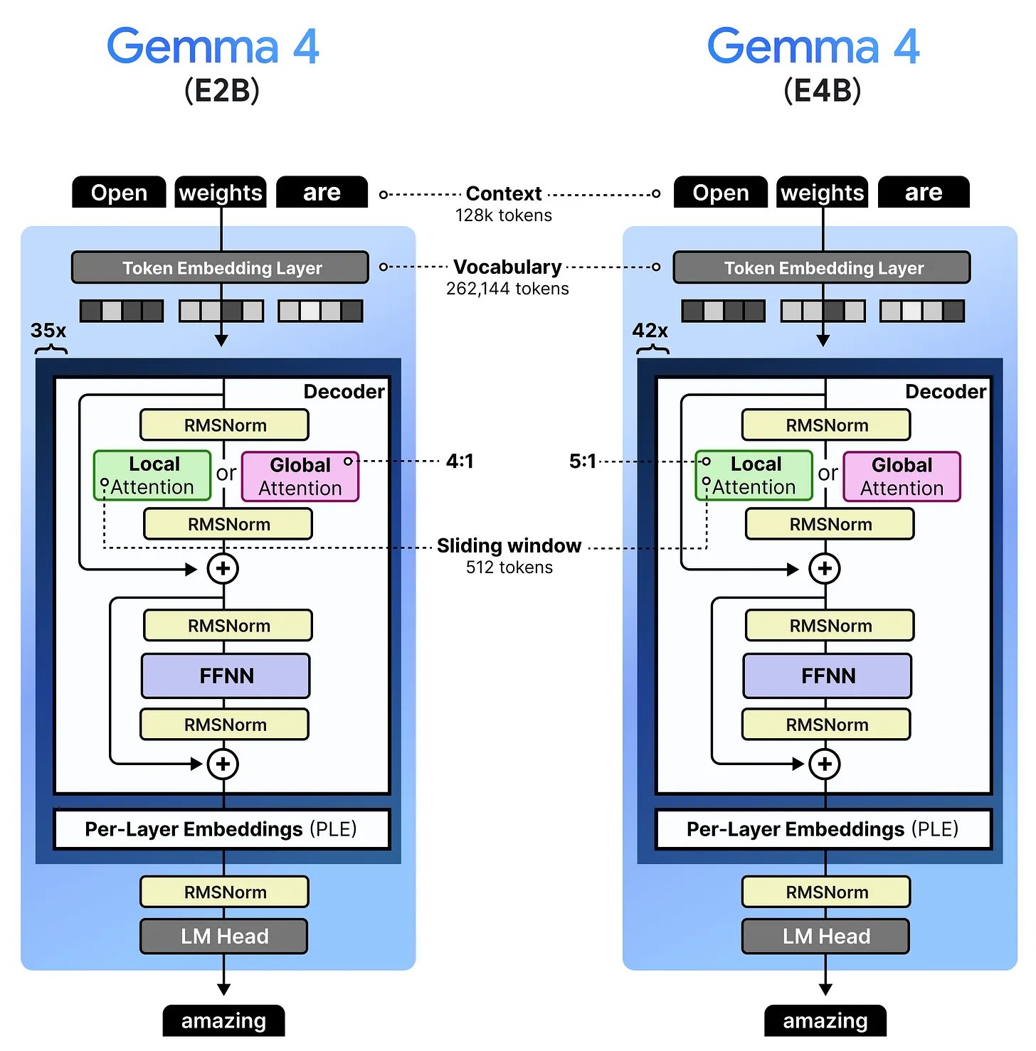The dark border is the PLE table — lives in flash storage, not RAM, injected fresh at every layer. — Maarten Grootendorst

The total parameter count of the PLE table is large (262,144 tokens × 35 layers × 256 dimensions for E2B). But none of it sits in RAM. The model's "effective" parameter count — the part that lives in RAM and does real-time computation — is just ~2B. That's where the "E" in "E2B" comes from.

It's a neat separation: use flash for storage-heavy stuff (lookup tables), keep RAM free for compute-heavy stuff (matrix multiplications). Phones have lots of flash and limited RAM, so the tradeoff lands well.

Audio in the small models

E2B and E4B are the only models in the family that handle audio. The pipeline follows the same principle as vision — convert a non-text input into embeddings that the language model can process alongside text — but the specifics are different because audio has different structure than images.

The raw audio waveform first gets converted into a mel spectrogram, which is a 2D representation with time on one axis and frequency bands on the other. If you've ever seen a colourful visualisation of an audio clip — that's roughly what a spectrogram looks like. This turns the audio signal into something that can be sliced into chunks and processed spatially.

Those chunks are then compressed through two convolutional layers to shorten the sequence (raw audio is extremely long in token terms — even a few seconds generates thousands of frames). The result is a manageable set of "soft tokens" that represent the audio.

These tokens are fed into a Conformer, which is a variant of the Transformer encoder. The key difference from a regular Transformer is an added convolution module between the attention and feedforward layers. Convolutions are good at picking up local patterns — in audio, that's things like individual phonemes or syllable boundaries. The attention layers handle longer-range structure like sentence rhythm and intonation. Combining both gives you an encoder that works well across audio timescales.

Finally, the Conformer's outputs get projected (same idea as with vision) into the embedding space Gemma 4 expects. At that point, audio, image, and text tokens all live in the same sequence and the model processes them uniformly.

Having text, vision, and audio in one small model is what makes the E-series interesting for on-device use. You don't need three separate models for three modalities — one model handles all of it, and it fits in phone RAM.

What ties it all together

I keep coming back to how specific each optimisation is. The Gemma 4 team didn't just make a bigger model and call it a day. Sliding window attention targets the quadratic cost of full attention. The GQA / K=V / p-RoPE stack targets the memory footprint of global attention specifically. MoE targets the gap between total model knowledge and per-token compute cost. PLE targets the RAM vs. flash distinction on mobile hardware.

Each fix is surgical, and they don't interfere with each other. That's what makes the family work — the same architectural base adapts cleanly to a 2B phone model and a 31B GPU model.

This post covers the main ideas. For the full technical detail — with many more diagrams — read Maarten Grootendorst's visual guide, which is where all the diagrams here come from.